YOLOX Explanation — Mosaic and Mixup For Data Augmentation
This article is the fourth and last in the series where I thoroughly explain how the YOLOX (You Only Look Once X) model works. If you are interested in the code, you can find a link to it below:
This series has 4 parts to fully go over the YOLOX algorithm:
- What is YOLO and What Makes It Special?
- How Does YOLOX Work?
- SimOTA For Dynamic Label Assignment
- Mosaic and Mixup For Data Augmentation (self)
Data Augmentation
Data augmentation is a way to help a model generalize. When augmenting data, the model must find new features in the data to recognize objects instead of relying on a few features to determine objects in an image.
YOLOX uses some of the best data augmentations to help the model generalize on the data more. I am going to talk about two of the best data augmentations YOLOX uses in this article.
Mosaic
The Mosaic data augmentation was first introduced in YOLOv4 and is an improvement of the CutMix data augmentation.
The idea behind Mosaic is very simple. Take 4 images and combine them into a single image. Mosaic does this by resizing each of the four images, stitching them together, and then taking a random cutout of the stitched images to get the final Mosaic image.
One of the difficulties when performing the Mosaic augmentation with the YOLO algorithm is that we have to worry about the bounding boxes when creating the final image. This task isn’t too hard as we can resize the bounding boxes and move them pretty easily. It’s just kind of annoying to figure out where the boxes should be moved after stitching the images together and creating the cutout.
The following are the steps to create the final Mosaic image given four images and the final size of the generated image:
- Resize the images. In this case, I am resizing to the shape of the output image
- Combine all images into a single image where each of the 4 resized images are a different corner
- Place the bounding boxes in the correct areas on the new image.
- Take a random cutout which is the size of the image we want the final result to be. This cutout can be anywhere on the combination of 4 images, but I put some restraints to make the final image a bit better
- Remove bounding boxes that aren’t in the cutout
- Resize any remaining bounding boxes that are cut off by the cutout
Let’s take a look at how this process works given the following 4 images and wanting a final image size of 256×256:

1. Resize the images to the final image size (256×256). This step can be done in many ways, but I do it by finding the image proportions and then manually resizing the image. The proportions come into play when resizing the bounding boxes since those need to be resized by the same proportion the image was resized. I have a function in my code called resize if you would like to see how I resized each image and its bounding boxes.

2. Combine all images into a single image. to do this, create a tensor of zeros which is of shape 3×512×512 and overlay each image onto each corner of the new tensor. Notice how in the image below all the bounding boxes are a mess, so we have to move them to their correct locations.

3. Moving the bounding boxes is easy enough:
- Bounding boxes for the top left image don’t have to be moved
- Bounding boxes in the top right image should be moved by 256 to the right
- Bounding boxes in the bottom left should be moved by 256 pixels down
- Bounding boxes in the bottom right should be moved by 256 pixels down and to the right
To move a bounding box by 256, just add 256 to either the x or y value in the bounding box array. Remember that each bounding box has 4 components (x, y, w, h)

4. Take a random cutout of the image.
One problem with just taking a random cutout anywhere on the image is the cutout tends to mostly contain one or two images, but we want it to contain all four images. To do this, we can take a cutout that can be anywhere within the square root of the final image dimensions (within 16 to 240). Although, the condition I set may be too small, but you can play around with the value constraints to find the condition you like.
The way I made the cutout was by selecting a random point between the square root of the final image dimension (16) and half the current combined image dimension minus the square root (240) to get the top left corner of the cutout. Then add on 256 to this random point to get the bottom right location of the cutout. This way, the cutout never goes beyond the max image dimension and stays within the square root boundary that we want the cutout to be in.

5. Remove bounding boxes outside the cutout.
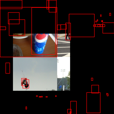
Notice how most of the bounding boxes lie outside the cutout area. To deal with this issue, we can first remove all bounding boxes outside of the cutout, but keep the ones that are even a little inside the cutout.

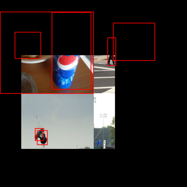
Notice how some bounding boxes still lie outside the cutout. We could’ve just gotten rid of these, but the problem with that technique is the model doesn’t learn what we want it to learn. We want the model to learn different features to differentiate different items, so we keep the bounding boxes that aren't completely in the cutout
6. Resize all remaining bounding boxes in the cutout
To deal with the remaining bounding boxes, we can resize them so that they are in the cutout. To do this, we can move all bounding boxes outside the cutout to be inside the cutout and then resize the bounding boxes by the amount we repositioned each bounding box. The final result looks like the following:

Notice how even the smallest of bounding boxes are kept in the image like the sandwich in the top left of the image. The model will have to generalize more to be able to recognize this object as a sandwich because this object doesn’t contain all the features your typical sandwich might contain.
I found an improved version of Mosaic which tackles problems with the Mosaic algorithm. If you wish to read more about it, you can find the paper at this link.
As for the original Mosaic algorithm, I couldn’t find a paper on it, but it was briefly introduced in YOLOv4 and there are a few sources online that talk about how the algorithm works.
Mixup
Mixup was originally created for classification tasks, but it still works really well for object detection tasks. Mixup basically averages two images together based on a weighting parameter λ. More formally, the paper describes defined Mixup by the following two formulas:

So, we can create an output image x̃ by combining two images xᵢ and xⱼ. But, since this augmentation was intended for label assignment, we also average the one-hot class embeddings as well. The task we want to solve has to do with bounding boxes, so instead of averaging the bounding boxes together, we just combine the annotations for both images into one. So all bounding boxes would be combined into the same list signifying all bounding boxes from both images also belong to the combined image.
The paper suggests sampling the λ parameter from a Beta distribution:

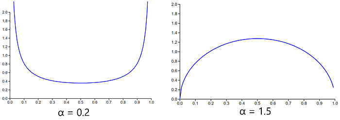
The paper shows results on α values at 0.2, 0.3, and 0.4, though I found that this led to an average that could lean on the higher ends of the spectrum toward 0 or 1. This means the image average wouldn’t really become the average of the two images and instead would be more like an image with some noise. I found somewhere online (I forget what site) that an α of 1.5 seemed to work better and came out with better-averaged images.

It looks like the Beta distribution at α = 1.5 favors values near 0.5 while the distribution at α = 0.2 favors values near 0 and 1.
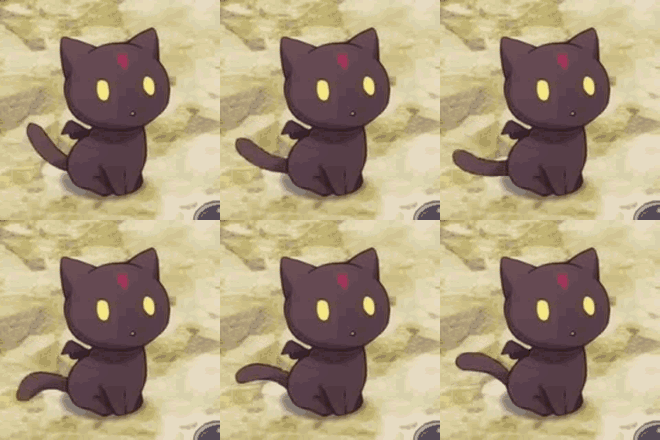
The result of Mixup has some interesting results and looks like the following:

The Mixup paper also goes into why Mixup works. If you wish to read about why Mixup works, I have linked to the paper at the end of this article.
Implementing Mixup for object detection isn’t difficult and requires some basic steps:
- Resize the images to be the same dimensions
- Sample from the Beta distribution to get the λ value
- Multiply all values in image 1 by λ
- Multiply all values in image 2 by 1-λ
- Add the two images together to get the final image
- Combine the annotations to get the final annotations for the image
If you wish to see how I implemented either Mixup or Mosaic, you can find it on my Github linked at the top of this article.
Mixup and Mosaic are the two big augmentations YOLOX uses. The idea behind both are relatively simple and aren’t too difficult to implement. This is the final article going over how YOLOX works. If you have any questions, please let me know and I will try to answer them.
References
YOLOv4: https://arxiv.org/abs/2004.10934
Mosaic Explanation: https://www.youtube.com/watch?time_continue=450&v=V6uj-eGmE7g&feature=emb_title
